
Dynamita, www.dynamita.com, Sigale, France
DYNAMIZU is one of the first dynamic simulators focused on water treatment processes. It was put together by a dedicated team with professionalism and thousands of days of tender loving care. Enjoy, and please let us know if you find somewhere it is coming short of your expectations. We will do our best to improve it.
Imre Takács, on behalf of the whole Dynamita team
Sigale-Toulouse-Budapest-Toronto-Québec-Luxembourg-Innsbruck
Released: January, 2026
Last updated: January, 2026
¶ Contact
This Quick Tutorial, the DYNAMIZU software, SumoSlang and related technologies are the copyright of Dynamita.
Copyright 2011-2026, Dynamita
Dynamita SAS
2015 route d’Aiglun
Sigale, 06910
France
www.dynamita.com
info@dynamita.com
support@dynamita.com
Mobile in France: +33.6.79.78.02.52
¶ Install DYNAMIZU
The following steps will help to guide you through the installation of DYNAMIZU.
¶ Prepare Microsoft Windows for DYNAMIZU
Operating system
Make sure your computer is operating Microsoft Windows 10 or later. DYNAMIZU supports touch screen computers running Windows 10 and 11.
DYNAMIZU can be used on a Mac with Windows installed or through an emulator like “Parallels”.
Microsoft Office
DYNAMIZU requires Microsoft Excel 2007 or later installed.
.NET
Please make sure that your computer is running the Microsoft .NET 4.7.2 framework. You can check it in the list of installed applications (Control Panel / Programs / Programs and Features). If the .NET framework’s 4.7.2 version is not installed, please download and install it from the following location:
https://dotnet.microsoft.com/download/dotnet-framework/net472
Windows 11 comes with the required .NET environment. On other operating systems, if you have it already installed on your computer, the downloaded installer will exit or inform you. Proceed to the next step.
¶ Installation of DYNAMIZU
You have received a link to the DYNAMIZU installer (or in rare cases the install file on a USB key). This is one file and contains everything necessary to install DYNAMIZU once Windows is prepared. Download it through the link provided to your computer. From the USB key you can install directly if desired, it is not required to copy the file to the computer.
Install DYNAMIZU by starting the install package and follow the instructions. Administrator rights may be required during installation. For workstations, we recommend choosing the “Install for myself only” option.
¶ Obtaining a license
Obtaining a license is a two-step process.
- After install, start DYNAMIZU from the Windows Start menu. DYNAMIZU will display a message providing multiple options. If you don’t have the license file yet, Select “I need a new license”. DYNAMIZU will display two additional buttons to show information about your hardware (DynaMic, Machine Identifier Code) and to copy this information directly to the Windows clipboard. Please paste this code into an email and send it to info@dynamita.com. Dynamita will provide a license file for you according to our agreement.
- Copy the license file Dynamita provided to a folder on your computer, start DYNAMIZU, choose the “I have a license” option, click “Select license file” and navigate to load the license file. As long as the license file is not deleted or moved and it is valid, this validation does not have to be repeated. Other options, like using a license server or a hardlock, are also available.
¶ How to build a plant
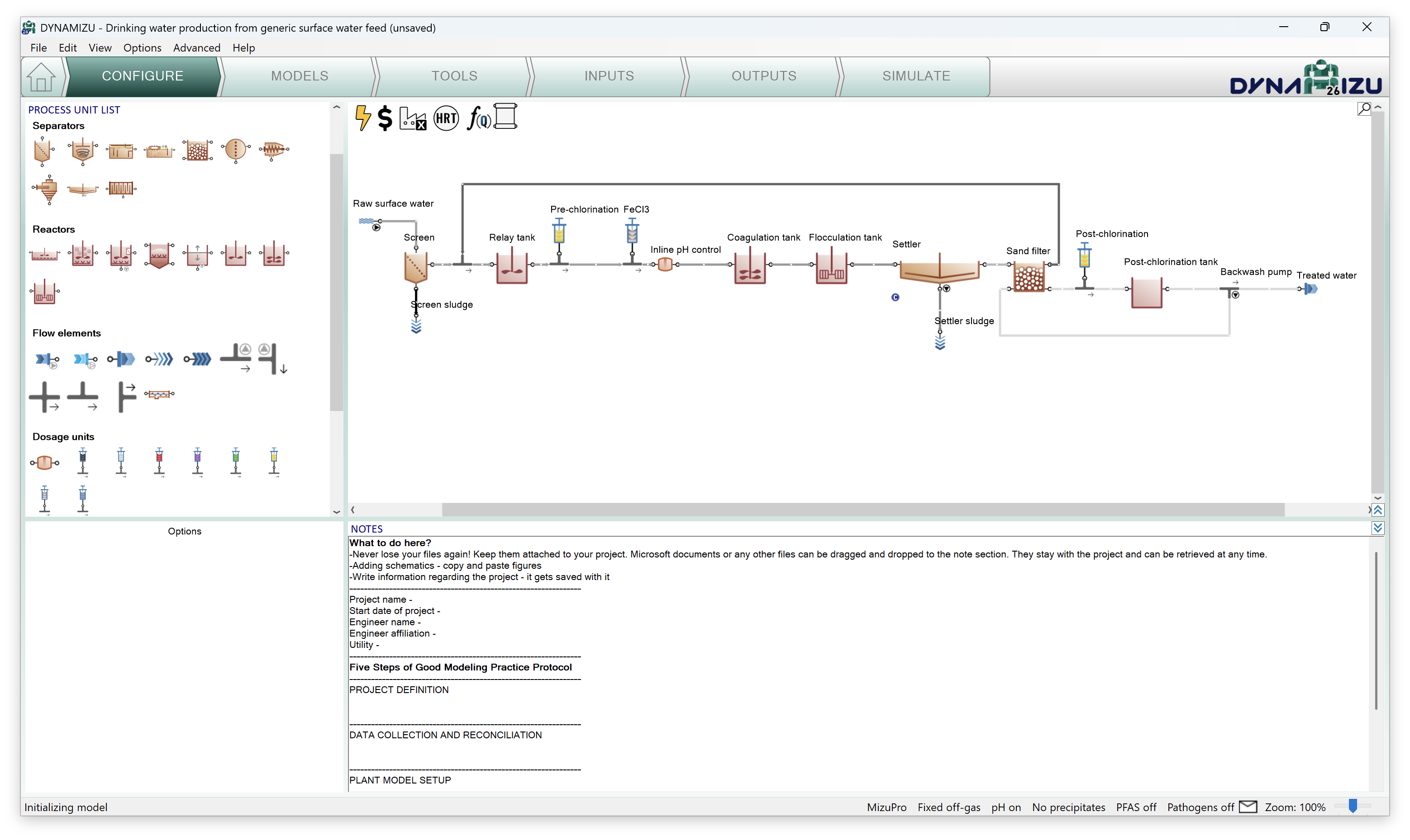
Start DYNAMIZU from the Desktop icon. DYNAMIZU will start with showing the Welcome Screen, as illustrated in Figure 1. Below the Menu Bar, you will see the Task Bar that guides you through the project workflow, all the way from configuration to simulation. The main window is split into four panels with various functionalities. The bottom strip is the status bar, showing the simulation status, the main model settings and messages from the GUI, if any.

¶ Configure
Click on the Configure tab. In this introduction, we will build a drinking water production plant configuration using different categories from the process unit list of the top left screen panel. Select the desired process unit by opening the category (just click on the category name to reveal the icons of available process units) and dragging the process unit to the drawing board (Figure 2). To drop the selected unit, just release the mouse button.
.png)
The units can be connected with pipes by simply positioning their outflow connection (port) on top of an input port of another process unit (Figure 3), or by positioning the mouse on an output port of a process unit, pressing the left mouse button, then moving the mouse – and this way dragging the pipe – to an input port of another process unit (Figure 4). Existing pipes can be removed by right-clicking on them and selecting Disconnect pipe from the pop-up menu.
.png)
.png)
Build the plant configuration and connect the pipes as shown in Figure 5. Rename (see Table 1 for the new names) or transform (rotate, mirror) the process units using the right-click pop-up menu. The pipes can be renamed as well, but this is usually not important – the pipe names are hidden by default (this can be changed in the View menu on the top). The visibility of process unit names can be controlled on a one-by-one basis.
The bottom left screen panel shows the different configurations that could be selected for each process unit (Figure 6 shows the options for the Feed as an example).

For this example layout, we will need to modify the names and the default configurations of a few process units as listed in Table 1.
Table 1 – Configuration setup for Conventional sand filtration with chlorination example
| Process unit category | Process unit name | Attribute group | Custom value |
| Flow elements / Feed | Raw surface water | Source of water | Lake |
| Measurement type | DOC based | ||
| Flow elements / Sludge | Screen sludge | Sludge type | Screening |
| Reactors / Storage tank | Relay tank | Reactions in storage tank | Reactive |
| Dosage units / Disinfection | Pre-chlorination | – | – |
| Dosage units / Metal | FeCl3 | Dosage specification at dosing point | Concentration of FeCl3 |
| Dosed chemical specification | Dosage based on the weight of the solution | ||
| Separators / Settler | Settler | Effluent specification | Percent solid removal |
| Flow elements / Sludge | Settler sludge | – | – |
| Separators / Sand filter | Sand filter | Effluent specification | Percent solid removal |
| Dosage units / Disinfection | Post-chlorination | – | – |
| Reactors / Storage tank | Post-chlorination tank | Reactions in storage tank | Reactive |
| Mixing | No mixer | ||
| Flow elements / Side flow divider | Backwash pump | – | – |
Note: the above settings can only be modified in Configuration mode, but you can return and perform them at any point during your work. Changing the process unit names will not result in recompilation of the project model.
Figure 7 shows the final layout, including modified process unit names and configurations.
.png)
¶ Models
The Models tab specifies which processes are included in the simulation. MizuPro is the model library developed for DYNAMIZU26. Additional considerations — gas phase calculations, pH, precipitates, micropollutants, and pathogens — can be enabled here. For this example, enable pH to be calculated (by selecting the Calculate pH option under the pH label) and Pathogens (by selecting the Pathogens are considered option) as demonstrated in Figure 8.
.png)
¶ Tools
Proceeding to the Tools tab, various calculations can be added to the simulation, ranging from HRT calculation to different types of controllers. In this example, a proportional flow dependency will be added by clicking the Proportional flow dependence button in the top left panel. The desired process units (or ports of process units) can be added to the respective slots of the dependence equation simply by dragging them from the drawing board. In this example, we are going to set the settler's sludge flow to be proportional to the raw surface water flow rate, as shown in Figure 9.
A blue “C” icon (for “Controlled”) will appear next to the settler on the drawing board, indicating that its sludge flow has become a dependent parameter controlled by another (in this case, the feed) flow. You can rename the FlowDependence tab to Settler's sludge using the right click menu.
The proportional dependency value can be defined in the subsequent step (Inputs). The controlling flow parameter (e.g., Raw surface water) is recommended to be external to the flow loop (if any are involved), as internal dependencies might create algebraically unsolvable systems due to the circular reference.
.png)
Note: When the project has at least one proportional flow dependency set up, the “Q” in the f(Q) icon on top of the drawing board gets a blue background.
¶ Inputs
Choosing the Inputs task, the green workflow tab above the drawing board automatically splits into Constants and Dynamics. Meanwhile, the model starts to be built (see bottom left message, in the status bar). For the initial plant setup, we will only need the Constants, as shown in Figure 10.
Once in the Inputs task, selecting each process unit will display a list of Input parameters at the bottom left panel. By default, only the most important ones are initially displayed. Clicking Show all in the bottom of the window panel reveals the rest of the list.
.png)
In this simple configuration, we only need to set a few values to build a realistic plant model. Use the custom values from Table 2 to set up the input parameters for this example. The process units not listed in the Table 2 should keep their default input values.
Table 2 – Input setup for Conventional Sand Filtration with Chlorination example
|
Process Unit |
Parameter group |
Parameter |
Custom value |
Unit |
|---|---|---|---|---|
| Raw surface water | Feed fractions | Colloidal fraction of DOC | 50 | % |
| Relay tank | Storage tank settings | Liquid volume per train | 1500 | m3 |
| Pre-chlorination | Dose specification | Chlorine concentration based dose | 1.2 | gCl2/m3 |
| FeCl3 | Dose specification | Dose by weight of stock solution per incoming flow | 15 | g/m3 |
| Post-chlorination | Dose specification | Chlorine concentration based dose | 0.2 | gCl2/m3 |
| Post-chlorination tank | Storage tank settings | Liquid volume per train | 500 | m3 |
| Backwash pump | Pump parameter | Pumped flow | 60 | m3/d |
Enter these values by selecting the respective process unit on the drawing board and the parameter group in the Input parameters menu (bottom left panel) – the values can be edited in the bottom right panel (Figure 10). Each value that is different from the default will be highlighted with bold letter type. There is also a similar indication in the Input parameters menu for parameter groups that contain non-default values.
For adjusting the flow dependency, select the f(Q) icon located in the top left region of the layout panel. The proportional flow parameter groups (Settler's sludge in this example) appear under Input parameters menu (bottom left panel). Set the input parameter as presented in Table 3.
Table 3 – Input setup for flow dependency in the Conventional sand filtration with chlorination example
|
Parameter group |
Parameter |
Custom value |
Unit |
|---|---|---|---|
| Settler's sludge | Settler's sludge proportion | 0.25 | % |
The input setup of this water treatment plant model is now ready. Meanwhile the model has compiled as well (status bar message: “Ready for simulation”).
The project can be saved any time during the configuration and project development using the File menu, and reopened at a later point in time.
¶ Outputs
This task can be used to specify which variables and in what format should be displayed and/or saved during the simulation phase.
For this example, add a table with the Flow and temperature, pH and Frequently used variables of the Raw surface water, Screen, Coagulation tank, Flocculation tank Output (port), Settler, Settler Sludge, Sand filter, Post-chlorination tank and Treated water process units (Figure 11); a timechart for Treated water nitrogen components (N) (Figure 12), a barchart for Total organic carbon (TOC) along the treatment plant (Figure 13). You can rename tables and charts by right-clicking on the desired tab, as illustrated in the Figures 11 to 13.
Select process units on the drawing board, and then drag and drop variables (or entire variable groups) from the bottom left panel (by default, variable groups are shown, clicking on the + icon will expand the group and list the variables in the selected group). You can also drag and drop process units to add new columns to an already existing table/barchart.
.png)
.png)
.png)
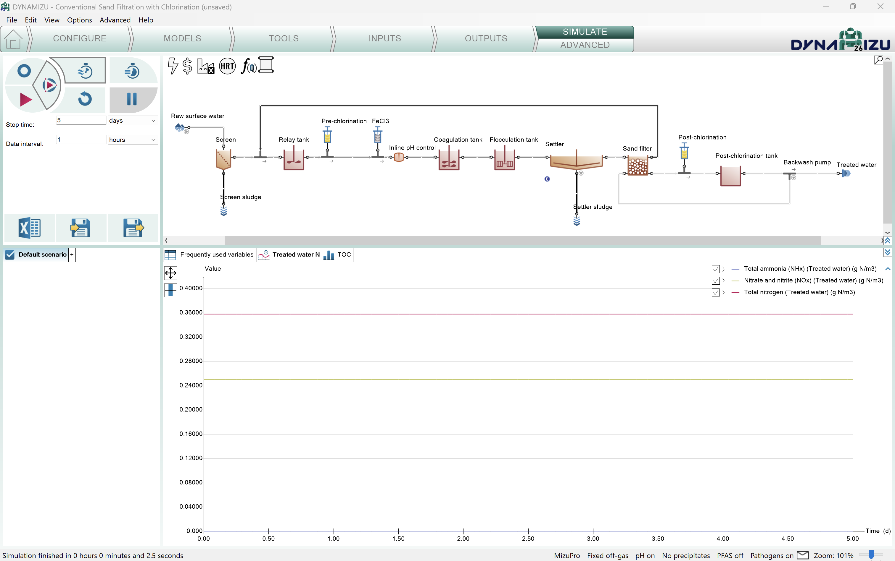
¶ Simulate
The last item on the Task Bar can be used to run simulations and observe the results (Figure 14). The simulation control panel in the top left window pane offers three modes that can be shuffled by a rotating circular button (hovering over the icons will reveal a descriptive label that helps identifying them). The Steady mode (blue circle icon) can be used to calculate directly the steady-state condition of the system, while using the Dynamic mode (red triangle) will show the variations with time, whereas the third, Dynamic from steady-state mode (blue circle with red triangle) will combine the two, starting a dynamic run from steady-state. The actually selected mode will be positioned on the right side of the circular button, highlighted by a slightly darker background color.
Four additional buttons are placed next to the simulation launchpad. In the top row you can toggle between two pre-configured solver settings: Fast (default) and Accurate, denoted by stopwatch icons. Usually the former is fast and accurate enough for most cases, and therefore its use is generally recommended. However, in certain situations (e.g. with biofilm models), the Accurate mode might provide faster simulation. Note that the mode selection will have effect on the steady-state solver as well. In the bottom row you can find the Reset and Pause/Continue buttons. The Reset button reinitiates the next simulation with the default concentrations defined in the model and process units. It should be employed thoughtfully, especially when working with complex plants, because reaching steady-state again might be time-consuming in these cases.
Saving and loading plant conditions (disk icons below the Stop time and Data interval fields) can be useful to restore system state (the actual values of the state variables) in case the simulation is driven into an unwanted condition (e.g. accidentally having been reset). Note that this function is not equivalent to saving the entire project (layout, model setup, tools, inputs and outputs) using the Save/Save as commands in the File menu.
.png)
The steady-state simulation employs different solvers to look for the steady-state condition of the system. In this mode, all dynamic inputs are disabled. The steady-state simulation will find the concentrations in the plant with constant influent and operating conditions, such as monthly average conditions etc. (Figures 15, 16 and 17). Note that the controllers are not set up for steady-state simulation.
.png)
.png)
.png)
Clicking on the Dynamic from steady-state button will initialize a steady-state run, followed by a dynamic run. The duration (Stop time) and the reporting frequency (Data interval) of the simulation can be set before the simulation (Figure 18).
Dynamic simulation can be started by pressing the red triangle button. Upon first start, the simulation will be started from the initial conditions (defaults specified in the model file and in the process units) and every subsequent run will be initiated with the last system state.
¶ Writing a report
Below the simulation control panel, a Report button is also available next to the Load/Save plant conditions buttons. When clicked, results of the last simulation will be written to an Excel file (saved with the same name as the DYNAMIZU project file by default) containing the following sheets:
- Project overview: contains the configuration layout and basic project information, as well as all the options selected for the MizuPro model
- Notes: the contents of the Notes screen panel from the Configuration tab
- Modified parameters: values of all parameters in the project that were changed from default
- Simulation results: all results of the output tabs get saved to separate sheets
- Plantwide calculations: Plantwide, Energy center, Cost center, HRT and Flow dependence settings
- Process Units: all settings and PU parameters are displayed on separate sheets for each unit
- Controllers: all settings and parameters of the controllers employed in the project (if any).
¶ Dynamic Inputs
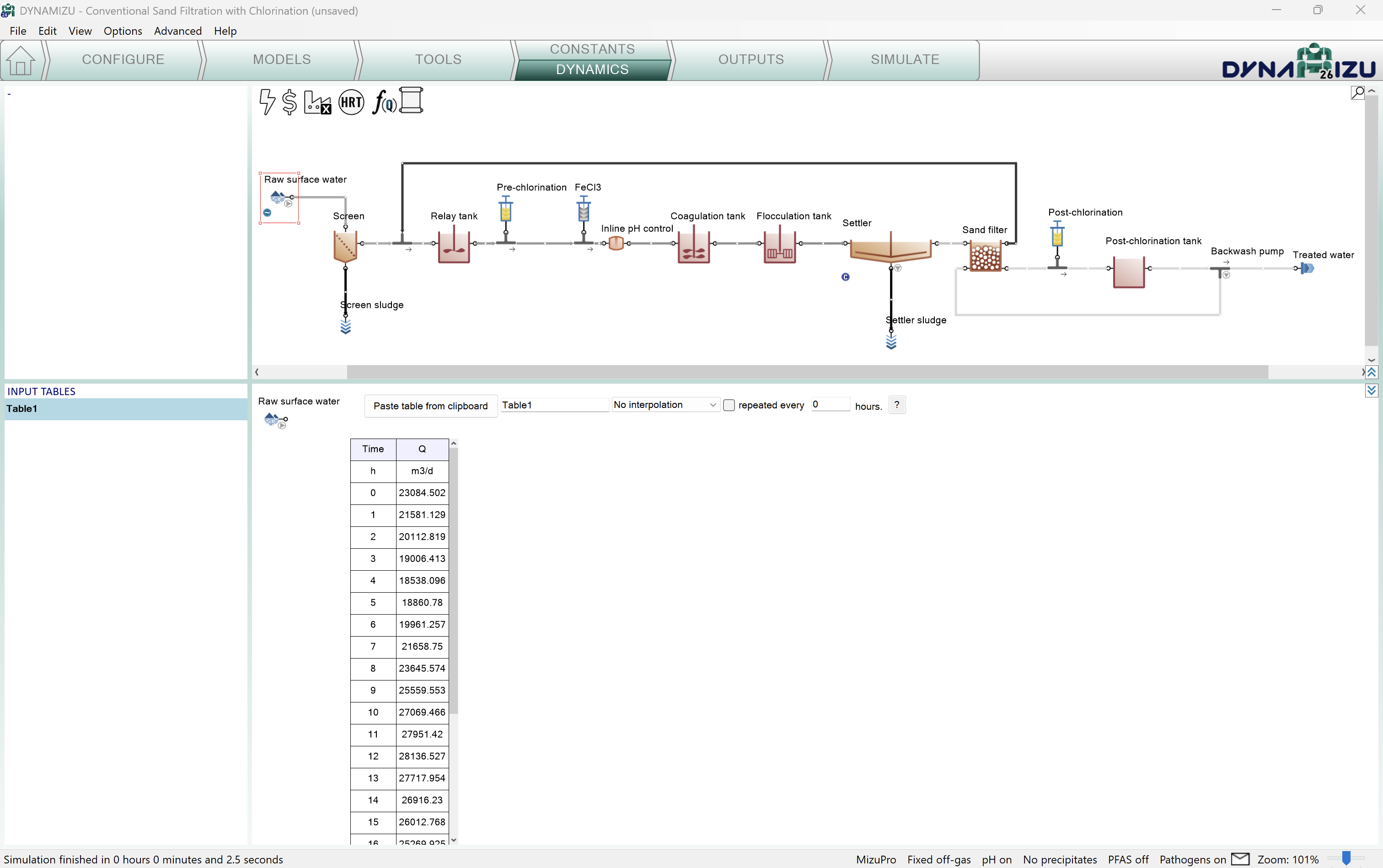
This optional task can be used to enter dynamically changing input information, e.g. diurnal flows, chemical dosage schedules and more. When choosing the Inputs tab, the green workflow tab automatically splits into Constants and Dynamics (Figure 19). According to this, different types of settings become available: we can set either constant inputs (e.g. fixed feed composition, metal dose specifications, and reactor volumes, as we just did) or dynamically changing inputs (e.g. variable Feed flow, composition, etc.).
Being on the Inputs/Dynamics tab, we can copy and paste prepared data tables from an Excel file into DYNAMIZU, simply by clicking on the Paste table from clipboard button when the desired process unit is selected (copy Table 4 over to an Excel spreadsheet, then copy it to Clipboard and paste into DYNAMIZU). This will apply the selected data ranges to the variables or parameters corresponding to the table headers (Figure 19). The latter have to comply with certain rules (More details will be provided in the future in the User Manual).
Table 4 – Dynamic input of feed flow pattern
| Time | Q |
|---|---|
| h | m3/d |
| 0 | 23084.502 |
| 1 | 21581.129 |
| 2 | 20112.819 |
| 3 | 19006.413 |
| 4 | 18538.096 |
| 5 | 18860.780 |
| 6 | 19961.257 |
| 7 | 21658.750 |
| 8 | 23645.574 |
| 9 | 25559.553 |
| 10 | 27069.466 |
| 11 | 27951.420 |
| 12 | 28136.527 |
| 13 | 27717.954 |
| 14 | 26916.230 |
| 15 | 26012.768 |
| 16 | 25269.925 |
| 17 | 24859.318 |
| 18 | 24817.715 |
| 19 | 25042.167 |
| 20 | 25325.377 |
| 21 | 25421.266 |
| 22 | 25122.513 |
| 23 | 24328.482 |
DYNAMIZU can simulate a wide range of operational scenarios, including more intricate reactor configurations and elaborate scenarios. These complex setups are available in the built-in example layouts.